
An Empirical Study with High Relevance in Medical AI Applications
Find all data of this study here.
Inhaltsverzeichnis
Abstract
Whether it’s X-rays of lungs or images of the eyeball – medical data sets are never perfect. A small number of misdiagnoses are often accompanied by a much bigger number of incorrect labels or annotations that can be traced back to incorrect documentation of the images. Using these erroneous data sets for training of convolutional neuronal networks affects the model’s classification quality. To investigate and quantify this effect, we artificially created a dataset with 100 percent correct labels and injected various ratios of corrupted labels into the training set. Finally, we measured the model performance on image classification. Results show more complex models generally to perform better. However, the decrease of model performance with increasing corrupted labels in training data does not solely depend on model complexity. In several cases, model performance plateaus and sometimes even slightly increases at very low levels of corrupted labels ratios. A strong correlation of model performance and corrupted labels ratio can be used as a potential basis to assess the unknown corrupted labels ratio in existing data sets.
Introduction
Computer vision already has a tangible impact in many industries. Especially in healthcare, the potential for the use of Artificial Intelligence (AI) is high. Algorithms and Convolutional Neural Networks (CNNs) have long been able to detect pneumonia (Patel et al. 2019; Rajpurkar et al. 2017; Stephen et al. 2019; Varshni et al. 2019), skin cancer (Esteva et al. 2017), malaria (Yang et al. 2017) and many other diseases with greater or at least the same accuracy as the best specialists in the respective field. Exemplary medical images used to train disease classification CNNs are shown in figure 1.
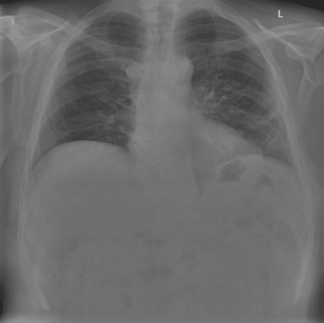

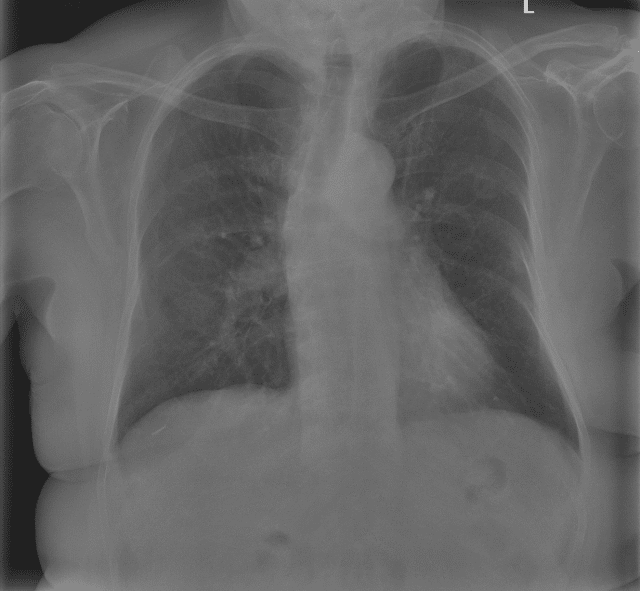
Figure 1: radiological imaging of COVID-19 patients (Winther et al. 2020) used for disease classification
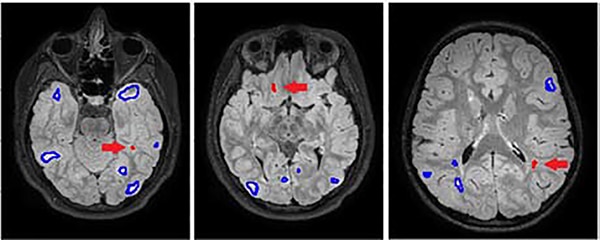
However, these models are subject to limitations because physicians often disagree markedly on the diagnosis of medical images. For example, in the evaluation of diabetic retinopathy. Doctors looked at images of the eyeball and classified the visual impairment on a scale of 1 to 5 as – in this order – full vision, slightly impaired, impaired, significantly impaired vision, and blind. The assessments of the medical experts often differ by several scales (Griffith et al. 1993; McKenna et al. 2018; Sussman et al. 1982). In addition, medical findings are occasionally documented incorrectly, or the labels (annotations interchangeably) are extracted from findings using NLP models. This adds further sources of error (Olatunji et al. 2019) in addition to potential incorrect diagnoses, for example in lung x-rays (Brady et al. 2012; Busby et al. 2018; Cohen et al. 2020; Oakden-Rayner 2019). Figure 2 shows example scans of tuberous sclerosis complex (TSC) patients with detected and missed annotations.
Humans are said to learn from their mistakes, which is true only if the errors are recognized. This can only marginally be applied to Artificial Intelligence. These algorithms depend on input data (often images in the medical field) being correctly labeled, i.e., given the right diagnoses, to produce the best performance on unseen data. The exact effect of incorrect labels in an image data set used to train self-learning algorithms is difficult to assess, but its overall negative impact on model performance has been proven and documented in various settings (Moosavi-Dezfooli et al. 2017; Pengfei Chen et al. 2019; Quinlan 1986; Speth und Hand. Emily M. 2019; Yu et al. 2018; Wang et al. 2018; Zhu und Wu 2004). In settings such as healthcare, each performance point won is valuable and potentially live saving.
In this work, we focus on studying the impairment of image classification on model performance due to corrupted labels (i.e., wrong label attribution of an observation) in the training data set. We artificially generate „diseases“ on images with the help of computer vision augmentation – and consequently label them 100% correctly without medical discrepancies. We then introduce and steadily increase the ratio of corrupted labels and measure the effect of the corrupted labels ratio (CLR) on model performance. Thereby, we hope to draw and generalize the conclusion of said effect for potential inference.
Background
Noisy label training
Deep learning neural networks in general as well as CNNs in specific are typically trained on large data sets with annotated labels. This process is called supervised learning. The source for errors in such data sets, which are used by the algorithm to learn certain relationships and patterns within the data, can be manifold and difficult to circumvent in many business settings. Often, correctly labeled data is cost intensive or generally difficult to obtain (Guan et al. 2018; Pechenizkiy et al. 2006) or labeling, even by experts, can still result in noisy data (Smyth 1996).
Other deep learning approaches to overcome these problems have already been explored, such as learning with noisy labels (Joulin et al. 2016; Natarajan et al. 2013; Song et al. 2022; Veit et al. 2017), self-supervised learning (Pinto et al. 2016; Wang und Gupta 2015) or unsupervised learning (Krizhevsky 2009; Le 2013 – 2013). These approaches and their measured performances demonstrate that deep learning models can tolerate some small amount of noise in the training set.
Multiple existing studies have probed the impact of noisy data on deep learning methods. These studies can generally be categorized into two groups (Rolnick et al. 2017). First, approaches that focus on noise-robust models to learn using noisy annotations (Beigman und Klebanov 2009; Joulin et al. 2016; Krause et al. 2015; Manwani und Sastry 2011; Misra et al. 2015; Natarajan et al. 2013; Reed et al. 2014; Rolnick et al. 2017; Liu et al. 2020). Some of these explicitly focus on image classification and CNNs (Ali et al. 2017; Xiao et al. 2015). This first group is comparatively bigger, as the noise-robust approach has more scaling potential as well as can optimally lead to a “train-and-forget” implementation of such models due to their robustness. Second, approaches that focus on identifying and removing or correcting corrupt data labels (Aha et al. 1991; Brodley und Friedl 1999; Skalak 1994). Karimi and colleagues provide an in-depth overview for various methods of both groups (Karimi et al. 2020).
Corrupted labels effect
Our study diverges from previous approaches, as the experiment is set up to have full control over the labeling process and thereby the data labels themselves. We then modify the CLR in the training data and consequently measure the changes of model performance. Furthermore, compared to other similar studies (Veit et al. 2016; Sukhbaatar et al. 2014), the model architecture used to train on the clean and then partially corrupted data is not changed. We likewise hope that focusing on the performance change, and not the performance level itself, will provide valuable insights.
The closest are two studies experimenting with incrementally changing the ratio of corrupted labels and its effect on model performance (van Horn et al. 2015; Zhang et al. 2016). The first of which finds that the increase of classification error due to label corruption in training data is surprisingly low, independent of the number of classes or computer vision algorithm. They conclude that for low CLRs (≤ 15%) the increase in classification error is smaller than the proportion of which the CLR is increased. When corruption is introduced not only to training data but also the test data set, a significant drop in model performance is found (van Horn et al. 2015). As model performance is measured based on CLR with large intervals (5%, 15%, 50%) we will extend on this study by using smaller intervals with a focus on the 0 % ≤ CLR ≤ 10% range. The second study independently corrupts the train labels based on a given probability with a stepwise increase of 10%, running the experiment with two different CNN architectures on two different data sets (Zhang et al. 2016). They conclude that label noise slows down the fitting convergence time with an increasing level of label noises. Again, we choose a more granular change in CLR and evaluate the magnitude of model performance change while using the same model architecture on the same data set across the different ratios. Thereby, we expect this to be a meaningful extension of these two studies.
Experiment
Data set augmentation and labeling
The base data set used is the public and freely available joined data sets PascalVoc from 2007 and 2012, where certain objects, such as people, bicycles, chairs, bottles, or sofas are originally labeled and annotated. Using these images as a basis, typical patterns in certain pathologies are artificially replicated onto the images. The focus is on ensuring that that these patterns are created to be unambiguous in certain cases, and barely or not at all recognizable to the human eye in others. Some of the results are shown in Figures 3a through 3c.

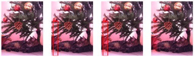
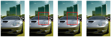

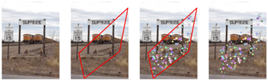

The respective image changes are based on two steps. First, a random image section is chosen, either as a rectangle or as a four-sided polygon. Then, within the selected image section, the pixel values of the image are randomly changed, and the images are labeled based on the type of pixel value change. The changes consist of four main classes and 14 subclasses as listed in table 1. For the corruption of labels, the annotation of an image is randomly changed to one of the not correct main or subclass respectively.
Main class (with description) | Subclasses |
|---|---|
| Distortion Pixel values in the region of interest are randomly changed within a specified interval. | · R: Red channel only · G: Green channel only · B: Blue channel only · All: All channels |
| Blur Pixel values in the region in question are blurred. | · No subclasses |
| Blob Random number of dots of random size are added to the region in question. | · R: Red dots · G: Green dots · B: Blue dots · All: Dots of random color |
| Color-X-Change In the region in question, the color channels are randomly swapped. | · RBG: RGB (red-green-blue sequence) becomes RBG · BGR: RGB becomes BGR · GRB: RGB becomes GRB · BRG: RGB becomes BRG · BBR: RGB becomes GBR |
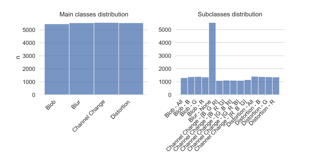
Overall, 22,077 pictures are altered and labeled. The distribution of main and subclasses is shown in figure 4. The distribution of main classes is roughly equal, with around 5,500 images per class. For subclasses, an imbalance is given due to Blur-class having no subclasses, resulting in ~ 5,500 images. For all other subclasses, between 1,100 and 1,400 pictures are altered and labeled. As this study focuses on change in model performance and not optimization of model performance or prediction performance of a certain class, the impact of class imbalance on overall performance will not be further discussed. All images including the created polygons are reseized after alteration to a pixel width and height of 244 before being loaded into the neuronal networks, resulting in an input shape of (244, 244, 3) .
Base and pretrained model architecture
Two models are used in the experiment setup. A self-developed, basic CNN (bCNN) with 7.2 million parameters as well as a pretrained ResNet50 (resnet) with 27.8 million parameters. The bCNN consists of nine convolutional layers, with each being encapsulated by batch normalization, pooling, and dropout layers (rate = 0.1) ). A quadratic kernel_size = 3 is selected and as activation function LeakyReLu with an α = 0.3 is implemented. After flattening, two hidden dense layers are added, again accompanied by batch normalization, dropout layers (rate = 0.1 ) and the LeakyReLu activation function (α = 0.3 ). For the output layer, softmax activation function is selected. The ResNet model (He et al. 2015) is extended with a single hidden dense layer (relu activation function) and an output layer using the softmax activation function. A detailed overview of the model architecture can be viewed on the provided GitHub.
Model training setup with increasing CLR
The neuronal networks are trained to classify the images across multiple experiment iterations. Within each iteration, the CLR is gradually increased within the training data and model performance is measured using an uncorrupted test set. The random split of training test data is 77.5% to 22.5%, resulting in 13,700 images for training and 4,952 for testing. During the model training phase, the training data is randomly split using 20% (3,425 images) of the training images for validation. The training of a single model consists of 20 epochs and batch size of 32. Each experiment iteration includes training both models on one of the classification tasks (either four main classes or 14 sub classes) for ten different CLRs with 0% ≤ CLR ≤ 10% .
Within each run, the higher CLR includes already corrupted labels from the previous ratio, i.e., 10% CLR includes all corrupt labels from the 7.5% CLR which includes all corrupt labels from the 5% CLR and so forth. 20 iterations are performed for each classification task, resulting in 800 trained models (see table 2) and >400 compute hours. Model classification performance was measured using accuracy, weighted average precision, weighted average recall, and weighted average f1-score.
| Experiment Parameter | Experiment Parameter States | No. of States |
|---|---|---|
| Model | bCNN, ResNet50 | 2 |
| Classification Task | Main class classification, subclass classification | 2 |
| Corrupted Labels Ratio | 0.0%, 0.25%, 0.5%, 1.0%, 2.0%, 3.0%, 4.0%, 5.0%, 7.5%, 10.0% | 10 |
| Training Iterations | 20 | 20 |
| = 800 models |
Results
CLR based model performance decrease
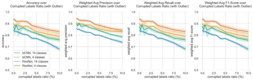
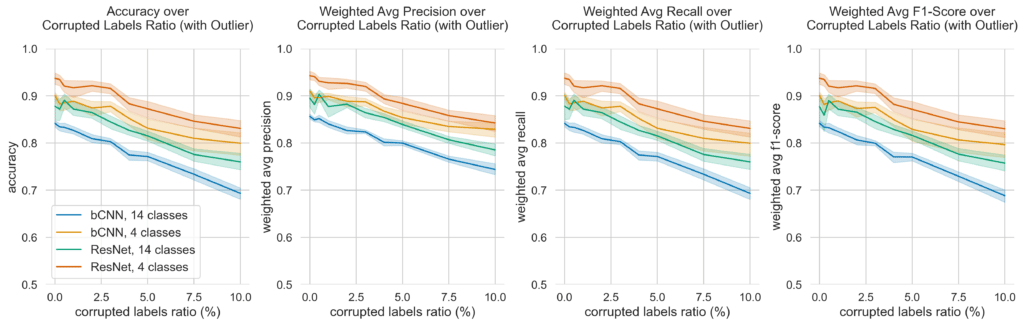
Overall, model performance decreased continuously with increase of CLR. An average test accuracy of 0.842 (std = 0.016) for the bCNN with 14 classes and 0% CLR is achieved, whereas 0.878 average accuracy (std = 0.064) is achieved by the ResNet model for the same classification task and CLR setup. The average accuracy decreases to 0.68 (std = 0.036 – bCNN, 10% CLR, 14 class prediction) and 0.76 (std = 0.04 – ResNet, 10% CLR, 14 class prediction).
* Number of removed model results using a z-score threshold of >3.0 calculated per metric – out off 800 model results: accuracy of 8 models removed, weighted avg. precision of 2 models removed, weighted avg. recall of 8 models removed, weighted avg. F1-score of 6 models removed
For four classes prediction, the bCNN average test accuracy with 0% CLR is 0.901 (std = 0.018). For the same setup (0% CLR, four class prediction), the ResNet achieves an average accuracy of 0.937 (std = 0.028 ). The average accuracy decreases to 0.789 (std = 0.072 – bCNN, 10% CLR, 4 class prediction) and 0.831 (std = 0.04 – ResNet, 10% CLR, 4 class prediction) respectively. Figure 5a gives an overview on the performance of the different model and classification task performances based on test data metrics.
Not only a steady decrease of more than 10 percentage points for each setup on the average accuracy can be observed, but also an increase of model performance variance as the CLR is increased. This behavior stays true for weighted average precision, weighted average recall and weighted average F1-score across all setups. A detailed overview can be found in appendix A.
Model performance anomalies of low level CLR
For the ResNet neural network trained on 14 classes prediction task, the standard deviation of accuracy, weighted average recall and weighted average F1-score is surprisingly high for an CLR of 0.0%, 0.25%, 0.5% and 1.0% when compared to the other setups (figure 5a, for details see appendix A). At the same time, an unusual characteristic is recognizable in the average performance change of the CLR for the 14 class ResNet: a peculiar spike in the test performance metrics when only a small number of labels are deliberately corrupted, i.e., at CLR = 0.5%. Even when removing outliers (see figure 5b), this pattern persists.
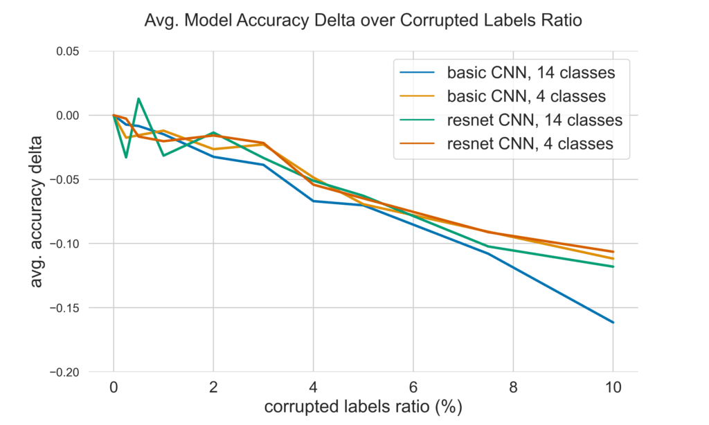
Figure 6 shows the average accuracy delta of each training setup compared to its average baseline (model trained with 0% CLR for same classification task). For both models, bCNN and ResNet, a further visual plateauing can be observed for the same low level CLRs (0.0% ≤ CLR ≤ 1.0% ) mentioned above when trained to classify four labels as well as the ResNet trained on 14 classes.
Classification performance relationship on CLR
A simple linear regression was run to probe the prediction of CLR based on a given accuracy, using the classification results as input. Table 3 confirms a moderately strong to strong negative correlation between the classification test accuracy (regressor) and the CLR (regressand) for all experiment setups with -0.75 ≤ r ≤ -0.5, except for the bCNN model trained on 14 classes with a very strong negative relationship of r < -0.9 .
| Model | Classification Task | Pearson’s r | p-value | Coefficient | RMSE train | RMSE test |
|---|---|---|---|---|---|---|
| bCNN | 4 classes | -0.64758 | < 0.00001 | -2.15962 | 2.39808 | 2.77765 |
| ResNet | 4 classes | -0.72335 | < 0.00001 | -2.32666 | 2.16245 | 2.31352 |
| bCNN | 14 classes | -0.90859 | < 0.00001 | -2.86965 | 1.37372 | 1.17014 |
| ResNet | 14 classes | -0.54147 | < 0.00001 | -1.51071 | 2.92637 | 2.16982 |
The coefficients, which can be interpreted as higher values indicating more robust models and lower ones indicating models that are more susceptible to false labels, shows the biggest effect of CLR on accuracy for the bCNN with 14 classes. While models used to choose and classify fewer number of classes achieve a better overall total accuracy performance, this observation does not automatically translate to a higher robustness of the models with respect to corrupted labels. Their performance decreases significantly faster than the ResNet trained to recognize 14 classes.
Discussion
With higher proportion of corrupted labels in the training data, model performance becomes less reliable. Performance declines faster than in previous similar studies (van Horn et al. 2015), which may be due to the overall comparatively low complexity of the model architecture used in the present study, as measured by the parameters that can be trained. Moreover, when fewer class types need to be classified by the model, performance is better across different CLR levels. This is likely because the differences in features, and thus underlying patterns used for class differentiation, are larger between main classes than between subclasses, especially between subclasses belonging to the same main class. It is plausible that as similarity increases (fewer differences in the underlying patterns), the predictive power of the model decreases regardless of the number of falsified labels.
Models with a higher number of trainable parameters perform better than those with fewer, across all CLR levels examined. The size of a network determines how much it can remember in terms of patterns observed during training. Here, a higher number of trainable parameters leads to improved recognition of patterns within images, as well as the relationship between these patterns and their respective classes. These results support previous research (Moosavi-Dezfooli et al. 2017; Pengfei Chen et al. 2019; Speth and Hand. Emily M. 2019; Wang et al. 2018; Yu et al. 2018; van Horn et al. 2015; Zhang et al. 2016). Since a model was implemented with pre-trained parameters, the potential for fine-tuning pattern recognition of already learned relationships was further increased. This is consistent with previous studies (Chandeep Sharma 2022; Hassan et al. 2021; Hussain et al. 2019; Wang et al. 2019).
An implication of the observed spike in performance at low CLR values for some of the experimental setups studied is that the model is better able to discriminate between frequent and less frequent patterns of correctly labeled images of the same class when the number of mislabeled images is extremely low. Thereby, robustness is increased for classification of unseen data by focusing on the most important class differences. As not all setups show this behavior, this implication cannot be concluded for certain.
Like the anomaly described above, the plateau in classification performance at the same low level of CLR allows for some interpretation. An inclusion of false labels does not immediately decrease pattern recognition of the models but potentially supports the identification of relationships between image and respective classes through pattern stimulation and emphasis on class differences. Only the model with the least trainable parameters per classes does not show described behavior and decreases steadily. Based on these observations, the conclusion might be drawn, that injecting a very low number of corrupted labels into the training data might increase model performance. The results suggest this to be feasible only if the model is complex enough in terms of trainable parameter per class ratio.
Based on the regression results, an initial estimate can be made about the existing corrupted labels in a dataset, even if the CLR is unknown. For instance, models trained on a dataset with uncertain CLR can be re-trained by intentionally inserting different ratios of falsified labels. Inferences can then be made about the data and its potential corrupted labels ratio used in the original model. The strong correlation between accuracy and CLR could potentially serve as an indicator for predicting the number of falsified labels and thus represents an interesting result for further research.
Conclusion
This study focuses on the effect of corrupted labels in training data for image classification models. We find, that more complex models generally perform better over various ratios of corrupted labels in the training data and across different classification task compared to lesser complex models. At the same time, results suggest that robustness does not automatically come with higher complexity of model architecture, as decrease of model performance does not seem to solely depend on model complexity. A surprising result is observed for one of the four training setups which opens further questions. Coming studies can draw on the present results and focus on performance plateauing and potential increase at very low levels of corrupted labels ratios, potentially as a source to overall improve model performance.
Data shows a case for using the strong relationship between model performance and corrupted labels ratio for inference of unknown CLR in existing data sets by deliberately inserting corrupted labels and measuring performance change. It is recommended to further validate this assumption by either increasing the number of model architectures measured or testing similar setups with different data sets.
Find all data of this study here.
References
- Aha, David W.; Kibler, Dennis; Albert, Marc K. (1991): Instance-based learning algorithms. In: Mach Learn 6 (1), S. 37–66. DOI: 10.1007/BF00153759.
- Ali, Tenvir; Jhandhir, Zeeshan; Ahmad, Awais; Khan, Murad; Khan, Arif Ali; Choi, Gyu Sang (2017): Detecting fraudulent labeling of rice samples using computer vision and fuzzy knowledge. In: Multimed Tools Appl 76 (23), S. 24675–24704. DOI: 10.1007/s11042-017-4472-9.
- Beigman, Eyal; Klebanov, Beata Beigman (2009): Learning with annotation noise. In: Keh-Yih Su (Hg.): Proceedings of the Joint Conference of the 47th Annual Meeting of the ACL and the 4th International Joint Conference on Natural Language Processing of the AFNLP: Volume 1 – Volume 1. the Joint Conference of the 47th Annual Meeting of the ACL and the 4th International Joint Conference. Suntec, Singapore, 8/2/2009 – 8/7/2009. United States: Association for Computational Linguistics (ACM Digital Library), S. 280.
- Brady, Adrian; Laoide, Risteárd Ó.; McCarthy, Peter; McDermott, Ronan (2012): Discrepancy and error in radiology: concepts, causes and consequences. In: The Ulster Medical Journal 81 (1), S. 3–9. DOI: Review.
- Brodley, C. E.; Friedl, M. A. (1999): Identifying Mislabeled Training Data. In: jair 11, S. 131–167. DOI: 10.1613/jair.606.
- Busby, Lindsay P.; Courtier, Jesse L.; Glastonbury, Christine M. (2018): Bias in Radiology: The How and Why of Misses and Misinterpretations. In: Radiographics : a review publication of the Radiological Society of North America, Inc 38 (1), S. 236–247. DOI: 10.1148/rg.2018170107.
- Chandeep Sharma (2022): Comparison of CNN and Pre-trained models: A Study. In:. Comparison of CNN and Pre-trained models: A Study. Available at https://www.researchgate.net/publication/359850786_Comparison_of_CNN_and_Pre-trained_models_A_Study.
- Cohen, Joseph Paul; Hashir, Mohammad; Brooks, Rupert; Bertrand, Hadrien (2020): On the limits of cross-domain generalization in automated X-ray prediction. Available at http://arxiv.org/pdf/2002.02497v2.
- Esteva, Andre; Kuprel, Brett; Novoa, Roberto A.; Ko, Justin; Swetter, Susan M.; Blau, Helen M.; Thrun, Sebastian (2017): Dermatologist-level classification of skin cancer with deep neural networks. In: Nature 542 (7639), S. 115–118. DOI: 10.1038/nature21056.
- Griffith, S. P.; Freeman, W. L.; Shaw, C. J.; Mitchell, W. H.; Olden, C. R.; Figgs, L. D. et al. (1993): Screening for diabetic retinopathy in a clinical setting: a comparison of direct ophthalmoscopy by primary care physicians with fundus photography. In: The Journal of family practice 37 (1), S. 49–56. DOI: Study.
- Guan, Melody; Gulshan, Varun; Dai, Andrew; Hinton, Geoffrey (2018): Who Said What: Modeling Individual Labelers Improves Classification. In: AAAI 32 (1). DOI: 10.1609/aaai.v32i1.11756.
- Hassan, Sk Mahmudul; Maji, Arnab Kumar; Jasiński, Michał; Leonowicz, Zbigniew; Jasińska, Elżbieta (2021): Identification of Plant-Leaf Diseases Using CNN and Transfer-Learning Approach. In: Electronics 10 (12), S. 1388. DOI: 10.3390/electronics10121388.
- He, Kaiming; Zhang, Xiangyu; Ren, Shaoqing; Sun, Jian (2015): Deep Residual Learning for Image Recognition. Available at https://arxiv.org/pdf/1512.03385.
- Winther, Hinrich B.; Laser, Hans; Gerbel, Svetlana; Maschke, Sabine K.; B. Hinrichs, Jan; Vogel-Claussen, Jens; et al. (2020): COVID-19 Image Repository. figshare. Dataset. https://doi.org/10.6084/m9.figshare.12275009.v1
- Hussain, Mahbub; Bird, Jordan J.; Faria, Diego R. (2019): A Study on CNN Transfer Learning for Image Classification. In:. UK Workshop on Computational Intelligence: Springer, Cham, S. 191–202. Available at https://link.springer.com/chapter/10.1007/978-3-319-97982-3_16.
- Joulin, Armand; van der Maaten, Laurens; Jabri, Allan; Vasilache, Nicolas (2016): Learning Visual Features from Large Weakly Supervised Data. In:. European Conference on Computer Vision: Springer, Cham, S. 67–84. Available at https://link.springer.com/chapter/10.1007/978-3-319-46478-7_5.
- Karimi, Davood; Dou, Haoran; Warfield, Simon K.; Gholipour, Ali (2020): Deep learning with noisy labels: Exploring techniques and remedies in medical image analysis. In: Medical image analysis 65, S. 101759. DOI: 10.1016/j.media.2020.101759.
- Krause, Jonathan; Sapp, Benjamin; Howard, Andrew; Zhou, Howard; Toshev, Alexander; Duerig, Tom et al. (2015): The Unreasonable Effectiveness of Noisy Data for Fine-Grained Recognition. Available at https://arxiv.org/pdf/1511.06789.
- Krizhevsky, Alex (2009): Learning multiple layers of features from tiny images. Available at http://www.cs.utoronto.ca/~kriz/learning-features-2009-tr.pdf.
- Le, Quoc V. (2013 – 2013): Building high-level features using large scale unsupervised learning. In: Acoustics, Speech and Signal Processing (ICASSP), 2013 IEEE International Conference on. ICASSP 2013 – 2013 IEEE International Conference on Acoustics, Speech and Signal Processing (ICASSP). Vancouver, BC, Canada, 5/26/2013 – 5/31/2013: IEEE, S. 8595–8598.
- Liu, Sheng; Niles-Weed, Jonathan; Razavian, Narges; Fernandez-Granda, Carlos (2020): Early-Learning Regularization Prevents Memorization of Noisy Labels. Available at https://arxiv.org/pdf/2007.00151.
- Manwani, Naresh; Sastry, P. S. (2011): Noise tolerance under risk minimization (3). Available at https://arxiv.org/pdf/1109.5231.
- McKenna, Martha; Chen, Tingting; McAneney, Helen; Vázquez Membrillo, Miguel Angel; Jin, Ling; Xiao, Wei et al. (2018): Accuracy of trained rural ophthalmologists versus non-medical image graders in the diagnosis of diabetic retinopathy in rural China. In: The British journal of ophthalmology 102 (11), S. 1471–1476. DOI: 10.1136/bjophthalmol-2018-312440.
- Misra, Ishan; Zitnick, C. Lawrence; Mitchell, Margaret; Girshick, Ross (2015): Seeing through the Human Reporting Bias: Visual Classifiers from Noisy Human-Centric Labels. Available at https://arxiv.org/pdf/1512.06974.
- Moosavi-Dezfooli, Seyed-Mohsen; Fawzi, Alhussein; Fawzi, Omar; Frossard, Pascal (2017): Universal Adversarial Perturbations. In: 2017 IEEE Conference on Computer Vision and Pattern Recognition (CVPR): IEEE.
- Natarajan, Nagarajan; Dhillon, Inderjit S.; Ravikumar, Pradeep K.; Tewari, Ambuj (2013): Learning with Noisy Labels. In: Advances in Neural Information Processing Systems 26. Available at https://proceedings.neurips.cc/paper/5073-learning-with-noisy-labels.
- Oakden-Rayner, Luke (2019): Exploring large scale public medical image datasets. Available at https://arxiv.org/pdf/1907.12720.
- Olatunji, Tobi; Yao, Li; Covington, Ben; Rhodes, Alexander; Upton, Anthony (2019): Caveats in Generating Medical Imaging Labels from Radiology Reports. Available at https://arxiv.org/pdf/1905.02283.
- Patel, Bhavik N.; Rosenberg, Louis; Willcox, Gregg; Baltaxe, David; Lyons, Mimi; Irvin, Jeremy et al. (2019): Human-machine partnership with artificial intelligence for chest radiograph diagnosis. In: NPJ digital medicine 2, S. 111. DOI: 10.1038/s41746-019-0189-7.
- Pechenizkiy, M.; Tsymbal, A.; Puuronen, S.; Pechenizkiy, O. (2006): Class Noise and Supervised Learning in Medical Domains: The Effect of Feature Extraction. In: 19th IEEE Symposium on Computer-Based Medical Systems (CBMS’06). Proceedings. 19th IEEE International Symposium on Computer-Based Medical Systems. Salt Lake City, UT: IEEE, S. 708–713.
- Pengfei Chen; Ben Ben Liao; Guangyong Chen; Shengyu Zhang (2019): Understanding and Utilizing Deep Neural Networks Trained with Noisy Labels. In: International Conference on Machine Learning, S. 1062–1070. Available at http://proceedings.mlr.press/v97/chen19g.html?ref=https://githubhelp.com.
- Pinto, Lerrel; Gandhi, Dhiraj; Han, Yuanfeng; Park, Yong-Lae; Gupta, Abhinav (2016): The Curious Robot: Learning Visual Representations via Physical Interactions. In:. European Conference on Computer Vision: Springer, Cham, S. 3–18. Available at https://link.springer.com/chapter/10.1007/978-3-319-46475-6_1.
- Quinlan, J. R. (1986): Induction of decision trees. In: Mach Learn 1 (1), S. 81–106. DOI: 10.1007/BF00116251.
- Rajpurkar, Pranav; Irvin, Jeremy; Zhu, Kaylie; Yang, Brandon; Mehta, Hershel; Duan, Tony et al. (2017): CheXNet: Radiologist-Level Pneumonia Detection on Chest X-Rays with Deep Learning. Available at http://arxiv.org/pdf/1711.05225v3.
- Reed, Scott; Lee, Honglak; Anguelov, Dragomir; Szegedy, Christian; Erhan, Dumitru; Rabinovich, Andrew (2014): Training Deep Neural Networks on Noisy Labels with Bootstrapping. Available at https://arxiv.org/pdf/1412.6596.
- Rolnick, David; Veit, Andreas; Belongie, Serge; Shavit, Nir (2017): Deep Learning is Robust to Massive Label Noise. Available at http://arxiv.org/pdf/1705.10694v3.
- Skalak, David B. (1994): Prototype and Feature Selection by Sampling and Random Mutation Hill Climbing Algorithms. In: Willian Cohen und Haym Hirsh (Hg.): Machine Learning. Proceedings of the Eleventh International Conference (ML 94). San Mateo, CA: Morgan Kaufmann, S. 293–301.
- Smyth, Padhraic (1996): Bounds on the mean classification error rate of multiple experts. In: Pattern Recognition Letters 17 (12), S. 1253–1257. DOI: 10.1016/0167-8655(96)00105-5.
- Song, Hwanjun; Kim, Minseok; Park, Dongmin; Shin, Yooju; Lee, Jae-Gil (2022): Learning From Noisy Labels With Deep Neural Networks: A Survey. In: IEEE transactions on neural networks and learning systems PP. DOI: 10.1109/TNNLS.2022.3152527.
- Speth, Jeremy; Hand. Emily M. (2019): Automated Label Noise Identification for Facial Attribute Recognition. Available at https://openaccess.thecvf.com/content_cvprw_2019/papers/uncertainty%20and%20robustness%20in%20deep%20visual%20learning/speth_automated_label_noise_identification_for_facial_attribute_recognition_cvprw_2019_paper.pdf.
- Stephen, Okeke; Sain, Mangal; Maduh, Uchenna Joseph; Jeong, Do-Un (2019): An Efficient Deep Learning Approach to Pneumonia Classification in Healthcare. In: Journal of healthcare engineering 2019, S. 4180949. DOI: 10.1155/2019/4180949.
- Sukhbaatar, Sainbayar; Bruna, Joan; Paluri, Manohar; Bourdev, Lubomir; Fergus, Rob (2014): Training Convolutional Networks with Noisy Labels. Available at https://arxiv.org/pdf/1406.2080.
- Sussman, E. J.; Tsiaras, W. G.; Soper, K. A. (1982): Diagnosis of diabetic eye disease. In: JAMA 247 (23), S. 3231–3234.
- van Horn, Grant; Branson, Steve; Farrell, Ryan; Haber, Scott; Barry, Jessie; Ipeirotis, Panos et al. (2015): Building a bird recognition app and large scale dataset with citizen scientists: The fine print in fine-grained dataset collection. In: 2015 IEEE Conference on Computer Vision and Pattern Recognition (CVPR). 7-12 June 2015, [Boston, MA, USA]. 2015 IEEE Conference on Computer Vision and Pattern Recognition (CVPR). Boston, MA, USA, 6/7/2015 – 6/12/2015. [Piscataway (NJ): IEEE Computer Society], S. 595–604.
- Varshni, Dimpy; Thakral, Kartik; Agarwal, Lucky; Nijhawan, Rahul; Mittal, Ankush (2019): Pneumonia Detection Using CNN based Feature Extraction. In: 2019 IEEE International Conference on Electrical, Computer and Communication Technologies (ICECCT). 2019 IEEE International Conference on Electrical, Computer and Communication Technologies (ICECCT). Coimbatore, India, 20.02.2019 – 22.02.2019: IEEE, S. 1–7.
- Veit, Andreas; Alldrin, Neil; Chechik, Gal; Krasin, Ivan; Gupta, Abhinav; Belongie, Serge (2017): Learning from Noisy Large-Scale Datasets with Minimal Supervision. In: 2017 IEEE Conference on Computer Vision and Pattern Recognition (CVPR): IEEE.
- Veit, Andreas; Wilber, Michael; Belongie, Serge (2016): Residual Networks Behave Like Ensembles of Relatively Shallow Networks. Available at https://arxiv.org/pdf/1605.06431.
- Wang, Fei; Chen, Liren; Li, Cheng; Huang, Shiyao; Chen, Yanjie; Qian, Chen; Loy, Chen Change (2018): The Devil of Face Recognition Is in the Noise. In: Vittorio Ferrari (Hg.): Computer vision – ECCV 2018. 15th European conference, Munich, Germany, September 8-14, 2018 : proceedingsnPart 9. Cham: Springer (Lecture notes in computer science, 11213), S. 780–795.
- Wang, Shui-Hua; Xie, Shipeng; Chen, Xianqing; Guttery, David S.; Tang, Chaosheng; Sun, Junding; Zhang, Yu-Dong (2019): Alcoholism Identification Based on an AlexNet Transfer Learning Model. In: Frontiers in psychiatry 10, S. 205. DOI: 10.3389/fpsyt.2019.00205.
- Wang, Xiaolong; Gupta, Abhinav (2015): Unsupervised Learning of Visual Representations Using Videos. In: 2015 IEEE International Conference on Computer Vision (ICCV): IEEE.
- Xiao, Tong; Xia, Tian; Yang, Yi; Huang, Chang; Wang, Xiaogang (2015): Learning from massive noisy labeled data for image classification. In: 2015 IEEE Conference on Computer Vision and Pattern Recognition (CVPR). 7-12 June 2015, [Boston, MA, USA]. 2015 IEEE Conference on Computer Vision and Pattern Recognition (CVPR). Boston, MA, USA, 6/7/2015 – 6/12/2015. [Piscataway (NJ): IEEE Computer Society], S. 2691–2699.
- Yang, Dahou; Subramanian, Gowtham; Duan, Jinming; Gao, Shaobing; Bai, Li; Chandramohanadas, Rajesh; Ai, Ye (2017): A portable image-based cytometer for rapid malaria detection and quantification. In: PloS one 12 (6), e0179161. DOI: 10.1371/journal.pone.0179161.
- Yu, Xiyu; Liu, Tongliang; Gong, Mingming; Zhang, Kun; Batmanghelich, Kayhan; Tao, Dacheng (2018): Transfer Learning with Label Noise: arXiv.
- Zhang, Chiyuan; Bengio, Samy; Hardt, Moritz; Recht, Benjamin; Vinyals, Oriol (2016): Understanding deep learning requires rethinking generalization. Available at https://arxiv.org/pdf/1611.03530.
- Zhu, Xingquan; Wu, Xindong (2004): Class Noise vs. Attribute Noise: A Quantitative Study. In: Artificial Intelligence Review 22 (3), S. 177–210. DOI: 10.1007/s10462-004-0751-8.
Appendix A – Classification metrics
| Model | Classes | Ratio (%) | Accuracy – mean | Weighted Avg. F1-Score – mean | Weighted Avg. Precision – mean | Weighted Avg. Recall – mean | Accuracy – std | Weighted Avg. f1-Score – std | Weighted Avg. Precision – std | Weighted Avg. Recall – std |
|---|---|---|---|---|---|---|---|---|---|---|
| bCNN | 14 | 0 | 0.841585 | 0.841569 | 0.856274 | 0.841585 | 0.015765 | 0.016428 | 0.011858 | 0.015765 |
| bCNN | 14 | 0.25 | 0.834243 | 0.833636 | 0.849078 | 0.834243 | 0.018119 | 0.016862 | 0.010445 | 0.018119 |
| bCNN | 14 | 0.5 | 0.833151 | 0.83232 | 0.851727 | 0.833151 | 0.023118 | 0.024443 | 0.017886 | 0.023118 |
| bCNN | 14 | 1 | 0.826751 | 0.824182 | 0.840438 | 0.826751 | 0.018587 | 0.020629 | 0.016899 | 0.018587 |
| bCNN | 14 | 2 | 0.80913 | 0.806645 | 0.826534 | 0.80913 | 0.020547 | 0.022943 | 0.018127 | 0.020547 |
| bCNN | 14 | 3 | 0.802899 | 0.799414 | 0.823501 | 0.802899 | 0.014477 | 0.012963 | 0.009651 | 0.014477 |
| bCNN | 14 | 4 | 0.774605 | 0.770601 | 0.801667 | 0.774605 | 0.023745 | 0.026735 | 0.017696 | 0.023745 |
| bCNN | 14 | 5 | 0.771367 | 0.77033 | 0.799715 | 0.771367 | 0.020306 | 0.018644 | 0.012359 | 0.020306 |
| bCNN | 14 | 7.5 | 0.73366 | 0.729435 | 0.765726 | 0.73366 | 0.026668 | 0.023696 | 0.015436 | 0.026668 |
| bCNN | 14 | 10 | 0.680102 | 0.678463 | 0.738586 | 0.680102 | 0.035719 | 0.03411 | 0.029199 | 0.035719 |
| bCNN | 4 | 0 | 0.90064 | 0.90043 | 0.909698 | 0.90064 | 0.016816 | 0.017951 | 0.011357 | 0.016816 |
| bCNN | 4 | 0.25 | 0.883076 | 0.881632 | 0.895888 | 0.883076 | 0.030711 | 0.033535 | 0.024019 | 0.030711 |
| bCNN | 4 | 0.5 | 0.885072 | 0.885436 | 0.896021 | 0.885072 | 0.034272 | 0.034266 | 0.02338 | 0.034272 |
| bCNN | 4 | 1 | 0.888554 | 0.88929 | 0.898819 | 0.888554 | 0.026146 | 0.024604 | 0.016208 | 0.026146 |
| bCNN | 4 | 2 | 0.874172 | 0.873042 | 0.888647 | 0.874172 | 0.035609 | 0.03735 | 0.024418 | 0.035609 |
| bCNN | 4 | 3 | 0.877805 | 0.875302 | 0.887272 | 0.877805 | 0.025013 | 0.028107 | 0.018683 | 0.025013 |
| bCNN | 4 | 4 | 0.85209 | 0.849806 | 0.867463 | 0.85209 | 0.032318 | 0.034461 | 0.022245 | 0.032318 |
| bCNN | 4 | 5 | 0.83125 | 0.828942 | 0.853832 | 0.83125 | 0.051635 | 0.055876 | 0.031775 | 0.051635 |
| bCNN | 4 | 7.5 | 0.809846 | 0.806584 | 0.835089 | 0.809846 | 0.057421 | 0.062427 | 0.027209 | 0.057421 |
| bCNN | 4 | 10 | 0.788874 | 0.785768 | 0.828895 | 0.788874 | 0.071561 | 0.075434 | 0.034534 | 0.071561 |
| ResNet | 14 | 0 | 0.877937 | 0.876813 | 0.894809 | 0.877937 | 0.063885 | 0.065784 | 0.044438 | 0.063885 |
| ResNet | 14 | 0.25 | 0.84503 | 0.846851 | 0.881667 | 0.84503 | 0.092582 | 0.08707 | 0.044718 | 0.092582 |
| ResNet | 14 | 0.5 | 0.890757 | 0.890049 | 0.903257 | 0.890757 | 0.035435 | 0.03872 | 0.024877 | 0.035435 |
| ResNet | 14 | 1 | 0.846404 | 0.842625 | 0.877276 | 0.846404 | 0.117977 | 0.133892 | 0.046202 | 0.117977 |
| ResNet | 14 | 2 | 0.864401 | 0.865366 | 0.882305 | 0.864401 | 0.028041 | 0.025746 | 0.017496 | 0.028041 |
| ResNet | 14 | 3 | 0.844635 | 0.845458 | 0.86419 | 0.844635 | 0.034156 | 0.034433 | 0.023673 | 0.034156 |
| ResNet | 14 | 4 | 0.826845 | 0.82875 | 0.85409 | 0.826845 | 0.024981 | 0.025226 | 0.019944 | 0.024981 |
| ResNet | 14 | 5 | 0.815136 | 0.816168 | 0.839149 | 0.815136 | 0.022655 | 0.021114 | 0.017676 | 0.022655 |
| ResNet | 14 | 7.5 | 0.77564 | 0.7764 | 0.806798 | 0.77564 | 0.03182 | 0.030592 | 0.017621 | 0.03182 |
| ResNet | 14 | 10 | 0.759902 | 0.757283 | 0.785185 | 0.759902 | 0.04012 | 0.039818 | 0.030053 | 0.04012 |
| ResNet | 4 | 0 | 0.937293 | 0.937203 | 0.942557 | 0.937293 | 0.028026 | 0.028343 | 0.021526 | 0.028026 |
| ResNet | 4 | 0.25 | 0.934601 | 0.934833 | 0.940729 | 0.934601 | 0.028955 | 0.02855 | 0.01846 | 0.028955 |
| ResNet | 4 | 0.5 | 0.920633 | 0.920504 | 0.930877 | 0.920633 | 0.029071 | 0.029474 | 0.019921 | 0.029071 |
| ResNet | 4 | 1 | 0.916999 | 0.917056 | 0.927508 | 0.916999 | 0.041602 | 0.041808 | 0.028402 | 0.041602 |
| ResNet | 4 | 2 | 0.92148 | 0.921242 | 0.926384 | 0.92148 | 0.02539 | 0.026496 | 0.021056 | 0.02539 |
| ResNet | 4 | 3 | 0.915644 | 0.915653 | 0.919914 | 0.915644 | 0.024833 | 0.02517 | 0.021372 | 0.024833 |
| ResNet | 4 | 4 | 0.883151 | 0.88214 | 0.893619 | 0.883151 | 0.032576 | 0.035687 | 0.023465 | 0.032576 |
| ResNet | 4 | 5 | 0.87244 | 0.871402 | 0.88391 | 0.87244 | 0.041492 | 0.043127 | 0.033444 | 0.041492 |
| ResNet | 4 | 7.5 | 0.846141 | 0.844722 | 0.858183 | 0.846141 | 0.034155 | 0.035994 | 0.026663 | 0.034155 |
| ResNet | 4 | 10 | 0.830873 | 0.830042 | 0.842399 | 0.830873 | 0.039727 | 0.040315 | 0.039217 | 0.039727 |


0 Kommentare