How to deal with missing values

Imputation methods and when they should be used

Why missing values matter

In our work as data scientists, we often work with time series data and applications for forecasting. As with all “classic” machine learning projects, forecasting often involves missing data that we have to deal with.

Missing values are particularly problematic for forecasting because the models usually contain time-dependent features. Time-dependent features are typically lagged or seasonal features. If the patterns of these features are interrupted, the models have difficulty learning these patterns. In addition, most classic forecasting methods, such as ARIMA models, cannot automatically handle missing values.

The first important step in dealing with missing values in time series is, as is so often the case, to analyze the data. These analysis steps can help determine whether the data is missing randomly or not. If values are not missing randomly and depend on the specific forecasting context, automated methods usually cannot handle the effects, and expert knowledge is required to deal with these cases.

An example of non-randomly missing data is the prediction of store sales, where data is always missing on holidays. On these days, sales are zero, and on the days before and after the holiday, sales typically increase. One method of addressing this issue could be to include features such as “holiday” or “day after holiday” in the model.

An example of random missing data could be accidents or errors that occurred during the transfer of data from the operational system to a data warehouse. These accidents were not dependent on the data and happened randomly at a specific point in time. If, on the other hand, it is an error that occurs regularly at certain times of the day or week, this would again be considered non-random missing data.

When performing the analysis, it is important to pay attention to the following details:

• What is the percentage of missing data in relation to the total volume?
• Do the gaps occur at regular intervals?
• How long are the gaps?

The most important methods of imputation and what to consider when using them

Most of the methods we list here are well known and have already been described in scientific papers and other online sources. In this article, we want to compare the different methods and provide guidance on when to use which method.

The first and by far the simplest method for dealing with missing data is to delete it.

This solution can be helpful for some classic machine learning problems, but not usually for time series. As mentioned earlier, this breaks the patterns in the time series and the model learns from incorrect patterns. Nevertheless, it is possible to select only the “healthy” part of the data set if this makes sense in terms of the desired goals. A practical solution could be to discard the first half of the data series if the quality improves from that point on (e.g., because the data collection process changed at a certain point in time). This option is only viable if we have enough data to train the models.

If deleting data is not an option, we must use some imputation methods, i.e., methods for filling in the missing values. One family of imputation methods uses the mean. The idea here is to fill in the missing values with the global, local, or seasonal mean to obtain a reasonable replacement value. Each of these methods is useful in different contexts, depending on the trend and seasonality of the data. Another option is to fill in the missing values with the previous or next available value, which is called forward or backward fill.

The last family of imputation methods we want to mention here is interpolation, i.e., inserting missing values into the observation range of a time series. This interpolation can be linear, polynomial, or spline, which defines the type of curve used to model the data. Linear interpolation can also be adjusted for seasonality (this is referred to as linear adjustment below). Another interpolation method is the use of Holt-Winters, a third-degree exponential smoothing that captures the level (first degree), trend (second degree), and seasonality (third degree) of the linear interpolation of the gaps.

The decision tree below summarizes our decisions and consolidates the rule of thumb we use most often. While this is a good starting point, we need to check with more accurate metrics and the eye test, i.e., we plot the values assumed by different methods to see which one best fits the pattern of the time series and helps the models make more accurate forecasts.

Evaluating the quality of imputation methods

To better understand the steps we typically follow when imputing missing values, let's look at a concrete example. Here, we start with a complete dataset and artificially generate missing values in order to compare the imputed values with the real ones. We used a dataset from the Store Item Demand Forecasting Challenge on Kaggle, which contains five years of sales data for 50 different items in 10 different stores. As mentioned earlier, the dataset is clean and contains no missing values. To reduce complexity, we aggregated the data to a monthly frequency.

We developed a function that randomly inserts a predefined percentage of missing values into the time series, with the option to parameterize the gaps (number and maximum length). With this function, we can try out different percentages of missing data and gap lengths. In this example, there are six gaps, with the longest being three months and 10% of the time series missing.

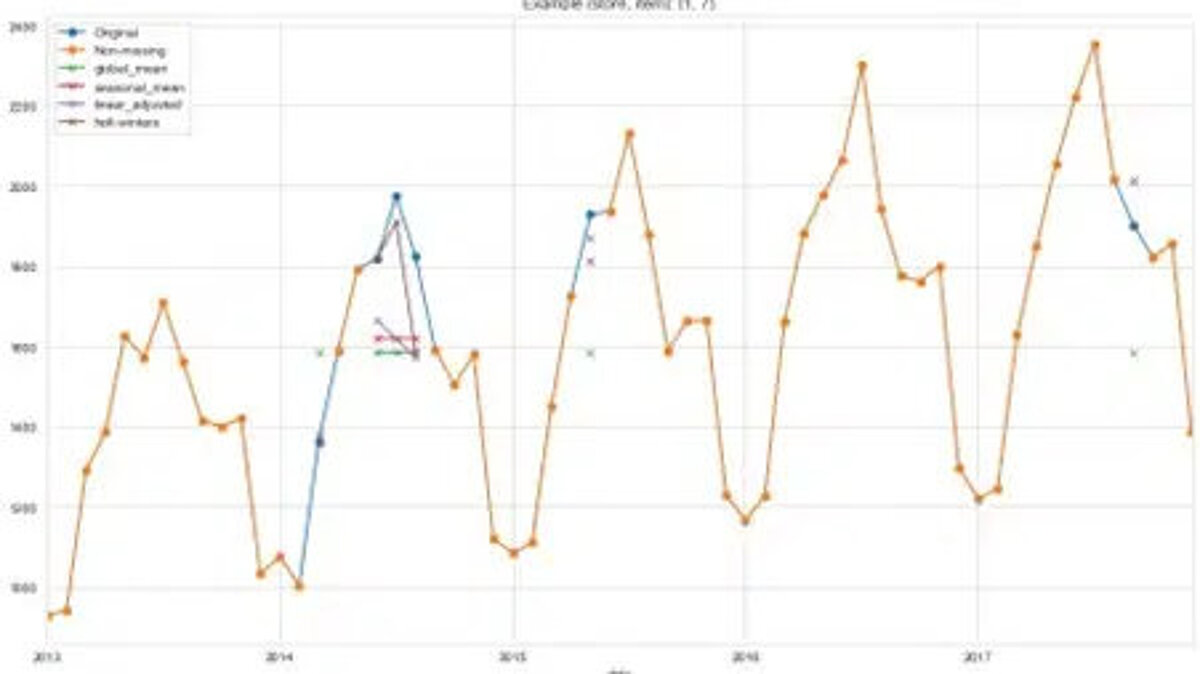
Now that the dataset contains missing values, we apply some of the methods listed above and compare them to the real data by visualizing them and comparing them with metrics. In the following example, we have only applied this to one of the time series from the dataset, whereas in a real project we would probably have to deal with many more time series.

The graph below shows the sales records for item 7 from store 1. The orange line describes the complete data available to us. The blue line shows the data we removed from the series for our experiments. The small crosses in different colors show the imputed values calculated using different methods. You can see that the linear fit and Holt-Winters imputation methods are better at capturing the variations in our time series. Because the data contains a trend and seasonality, the two methods that take trend and seasonality into account perform best. This confirms the rule of thumb we presented in the figure above.

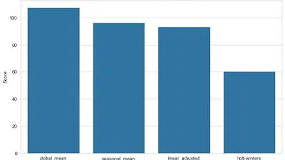
Since our goal is to achieve the best prediction result for future periods, we want to measure the impact of different imputation methods on a prediction model. Therefore, we fitted the same forecast model for each method and compared the errors for the test set (the last year of the series) using the following classic regression evaluation metrics:

• The symmetric mean absolute percentage error (sMAPE) or the mean absolute deviation in percent, which expresses accuracy as a ratio. It is very intuitive but can become very large due to a small error deviation (with a series of small denominators).
• The mean absolute error (MAE), which measures the distance between each forecast and the actual value, is easier to interpret.

The results of the forecast model for the various imputation methods are shown below. As already indicated in the chart above, the Holt-Winters method and the linearly adjusted imputation provide better forecast results than the mean value method. However, it also shows that the results of the seasonal mean method are comparable to those of the linearly adjusted method. This confirms that several methods should be tried and compared rather than relying solely on the rule of thumb. We also see that both metrics show the same result, which reinforces our conclusion.

Of course, this was only a model for a time series, and in a realistic example we would normally try out different forecast models for different time series. In this article, we wanted to focus on the different methods of imputation and their evaluation.

Conclusion & tips for application

In summary, it can be said that you should always start with an analysis of the time series data and examine whether the data is missing randomly or whether there are certain patterns. In the latter case, you should try to find explanations using your own expertise or by consulting experts in the field.

For example, during data analysis, you should ask yourself whether gaps occur at regular intervals, how long the gaps are, and what percentage of the total data is missing. The answers to these questions will often provide insight and help you find either specific solutions or suitable imputation methods according to our rule of thumb.

Even though the rule presented here is a good starting point for choosing the appropriate imputation method, it is also necessary to always evaluate it carefully. As with any forecasting model, it is extremely important and helpful to combine a visual evaluation with an analytical one.

During the visual evaluation, you should pay attention to which method best fits the pattern of the time series. For the analytical evaluation, the imputed values from different imputation methods can be used to train forecast models and evaluate them on a test set of data. This approach makes sense because the goal of imputation is to achieve good forecast results. Common forecasting metrics such as MAE or SMAPE can be useful for evaluation, but the appropriate metric always depends on the specific business objectives.