Reinforcement Learning: Example and Framework

What is Reinforcement Learning?

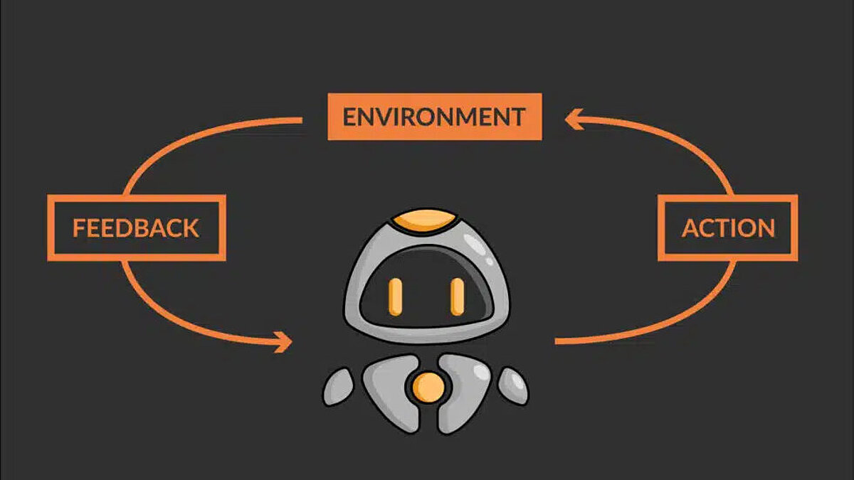
Reinforcement learning (RL) is a type of machine learning. It involves training agents to make decisions in an environment by learning from the consequences of their actions. The agent receives feedback in the form of “rewards” or “punishments,” which it uses to update its decision-making strategy and improve its performance over time. The agent learns through trial and error, i.e., it tries out different actions and receives feedback in the form of rewards or punishments. RL can be used for any process or system that involves a sequential decision-making process that could be optimized.

RL is used in areas such as autonomous driving, robotics, control systems, game AI, and economics and finance, e.g., in optimizing decision-making in portfolio optimization and resource allocation. It has also been used to improve the performance of dialogue systems (chatbots) such as ChatGPT, which have caused quite a stir in recent months.

Reinforcement Learning – Example & Definitions

This section provides an overview of the definitions and descriptions of the most important terms required to understand the dynamics of RL algorithms. It is always easier to understand complex terms using a simple visual reinforcement learning example, so we will explain the various terms below using a simple reinforcement learning problem.

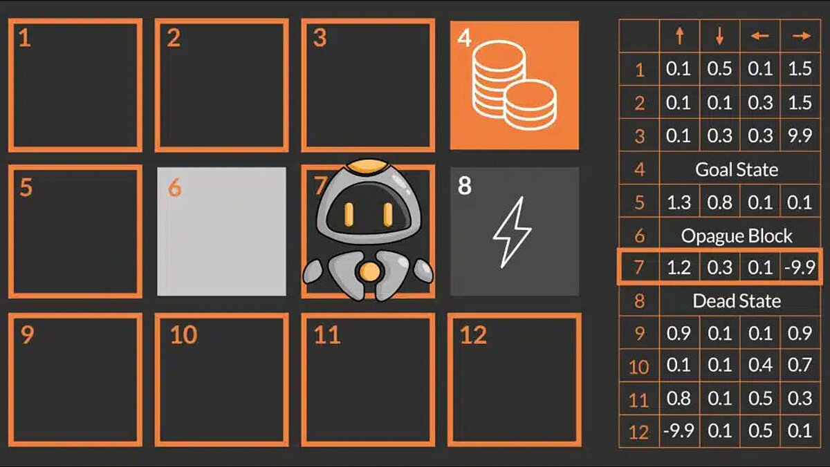
The main goal of our robot QT is to win the game by reaching the target field (also known as the target state), which is marked by coins, by finding and following the optimal path. To move around the maze, QT can perform four actions: go up, go down, go left, and go right. In this environment, there are some obstacles such as the lightning field and the impassable block (gray box). These obstacles can either kill QT or prevent it from performing its intended action (movement). Since QT has no prior knowledge of the maze, the idea is that QT tries to explore the environment by navigating randomly and finding a possible path to the goal.

To better understand how QT can achieve this, it is important to understand some basic RL components and terms that are also used to formulate the problem mathematically.

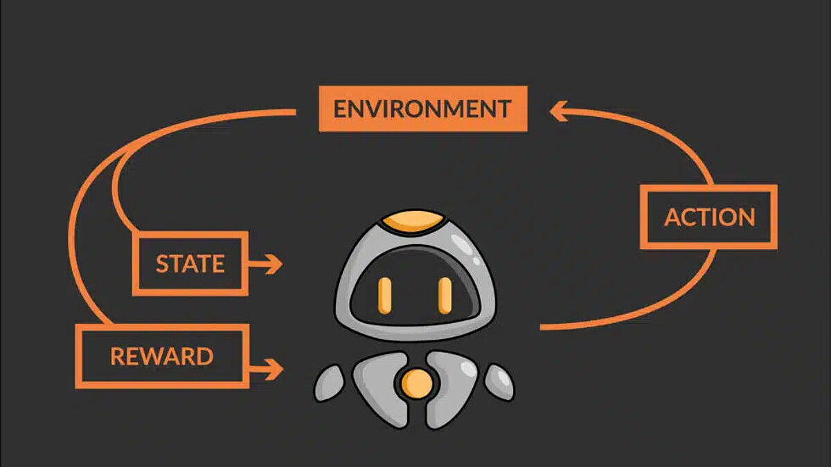
The maze is referred to as the environment and the robot QT as the agent. In reinforcement learning, the environment is the system, simulation, or space in which the agent can act. The most important thing is that the agent cannot change the rules or dynamics of the environment in any way. The environment is the world in which the agent interacts by performing certain actions and receiving feedback. The agent interacts with the environment and makes decisions. This can be a robot, a software program, or another system that can perform actions and then receive a reward. In the example above, QT (the RL agent) interacts with the maze (environment) by moving in one of the directions and updating its position in the maze. Below are the various components and characteristics of agent-environment interaction:

Reinforcement Learning Fundamental Definitions

1. State: The parameters or observations that describe the agent's environment are collectively referred to as the state of the environment. It includes everything the agent can observe about the environment, as well as all internal variables of the agent that may be relevant to the agent's actions. In the reinforcement learning example above, the state of the robot is its position in the maze. Some environments, such as the example above, have special states called terminal states, which include the target state (coin field) and other end states (lightning field). A terminal state is the state of the environment in which the agent is unable to continue. In this case, the agent ends its current learning cycle and a new learning cycle begins with the newly acquired knowledge about the environment.
2. Action: An action is a decision made by the agent and represents the agent's means of interacting with the environment. It can be a physical movement, a change in the agent's internal state, or any other type of decision that the agent can make. The consequences of the actions performed by the agent are the change in the state of the environment and the feedback it receives. In the reinforcement learning example above, our robot has four possible actions (up, down, left, or right) that it can perform to change its state.
3. Reward: When an agent performs an action, the environment not only provides feedback in the form of the new state, but also a reward signal. A reward represents the benefit that the agent gains from entering the new state based on its last action. The reward component is of utmost importance in RL, as it guides the agent in finding the optimal path or process. The concepts in the next section explain that the agent essentially tries to maximize the cumulative reward it receives from the environment in order to find the shortest path, as in the QT example above. In the example, the reward for the agent that enters the target state (coins) is +10 points, the reward for the agent that enters the lightning field is -10 points, and for all other states it could be 0 or -1 point.
4. Transition Probability: This is one of the most important properties for some environments. It defines the probability of moving from one state to another by performing a certain action in the current state. This parameter determines whether the environment is stochastic or deterministic. Accordingly, the agent's behavior in the same environment may vary. An example makes this concept easier to understand.
   • Deterministic environment: For such environments, the transition probability is set to 1. This means that the agent's transition from one state to another is determined solely by the action it performs in the current state. If QT decides to move to the right in the following example, it would land in the lightning field and definitely die! If, on the other hand, it decides to move up, it would be one step closer to the target state. For the rest of this article, the environment will remain deterministic.

• Stochastic environment: In such environments, the transition of the agent from one state to another is determined by the action it performs and by the distribution of transition probabilities, which determines which states it can transition to. The transition probabilities can be defined as follows (from the frozen lake problem): The agent moves with a probability of 1/3 (33%) in the direction it intends to move or with the same probability of 1/3 (33%) in a perpendicular direction, as shown below. Assuming that QT decides to move to the right, the probability of landing in the lightning field is 33% and of landing in one of the two blocks above and below is 33% each. This means that, unlike in the above environment, where it must avoid moving to the right at all costs in order to survive, QT can now take action to move to the right, as this offers a 66% chance of survival.

1. Exploration vs. exploitation: In RL, exploration and exploitation are two concepts that refer to the balance between trying out new actions to explore new states (exploration) and taking the best known action in the current state (according to QT's current assignment) to achieve the greatest possible reward (exploitation).

During the exploration phase, the agent tries out new actions to learn more about the environment and improve its decision-making. This helps the agent discover high-reward states and perform actions to reach them. In the exploitation phase, it tries to reach the final states in the optimal way to maximize the cumulative reward. In the reinforcement learning example above, QT would first try out actions to discover different states and possible paths to the goal. Sometimes it will end up in the lightning field and sometimes in the coin field, but it will gather knowledge and learn which state-action combinations lead to these states. With increasing experience, it will gradually learn to find the optimal path (in our example, the shortest path).

The balance between exploration and exploitation is often referred to as the exploration-exploitation trade-off. In general, the more an agent explores, the more knowledge it gains about the environment, but it may take longer to obtain the highest reward and find the optimal strategy. On the other hand, the more an agent exploits, the faster it can achieve a higher reward, but it does not necessarily find the optimal strategy and misses out on discovering very rewarding states. The following describes some common strategies that help strike a balance between exploration and exploitation:

• Epsilon-greedy algorithm (ε-greedy) In this algorithm, the agent starts with a high exploration probability (ε) and a low exploitation probability (1-ε). This allows the agent to explore new actions initially and gradually exploit the best known actions from experience. The rate of change of the value of ε is a hyperparameter that depends on the complexity of the RL problem. It can be defined linearly, exponentially, or by a mathematical expression.
• Upper Confidence Bound (UCB): In this algorithm, the agent selects an action based on the balance between the expected reward and the uncertainty of the action. This allows the agent to explore actions with high uncertainty, but also to exploit actions with high expected rewards. In UCB, the agent maintains an estimate of the expected reward of each action as well as a measure of the uncertainty of the estimate. The agent selects the action with the highest “upper confidence bound” value, which is the sum of the expected reward and a term representing the uncertainty of the estimate. The uncertainty term is often chosen as the square root of the natural logarithm of the total number of actions chosen. The intuition behind this is that the uncertainty of the estimate should decrease as the number of actions chosen increases, since the agent has more data on which to base its estimate.

Mathematical Formulation of Terminology using the Reinforcement Learning Example

Now that we have learned the basic terminology related to the “maze problem,” let's formulate and understand this terminology from a mathematical perspective.

1. The robot QT (agent) receives the state S₀ from the environment – the current block of the robot in the environment
2. Based on this state S₀, QT (agent) performs an action A₀ – let's say QT moves up
3. The environment changes to a new state S₁ – new block
4. The environment gives the agent a reward R₁ – QT is not dead yet (positive reward, +1)
5. The transition probability is denoted as P(S₁ | S₀, A₀) or T – here it is 1, since the environment is deterministic by nature

The loop above represents one step taken by the agent. The agent must take several such steps {S₀, A₀, R₁, S₁, T₀} to explore its environment and identify the good and bad states along with the actions that lead to them. Finally, it must navigate the optimal path to the goal.

In order to formulate and solve a decision-making or optimization problem using reinforcement learning, some very important concepts and terms must be explained.

In our deep dive, we shed light on the interactions between business methods, neuroscience, and reinforcement learning in artificial and biological intelligence.

Reinforcement learning – algorithms in the brain

DISCLAIMER: Now begins a mathematical deep dive!

Mathematical Modeling of a Decision Problem

1. Markov Decision Process = MDP: A Markov decision process is a process in which future states depend only on the current state and are in no way connected to the past states that led to the current state. This mathematical framework is used to model decision problems in reinforcement learning. Given a sequence of states, actions, and rewards s0, a0, r0, s1, a1, r1, s2, a2, r2....st, at, rt (the so-called history) observed by an agent, the state signal is said to have the Markov property if it satisfies the following equation:

P (S_t+1 = s′, R_t+1 = r′| s_t, a_t) = P (S_t+1 = s′, R_t+1 = r′| s_t, a_t, r_t, … s₀, a_0, r₀), where:

• S is a set of states, S = {s0, s1, …}
• A is a set of actions, A = {a0, a1, …}
• T is a set of transition probabilities, T = {P(st+1|st, At), P(st+2|st+1, At+1), P(st+3|st+2, At+2), …}
• R is a set of rewards, R = {r0, r1, …}

2. Cumulative Return and Discount Factor

a) RL agents learn by selecting an action that maximizes the cumulative future reward. The cumulative future reward is called the return and is often denoted by R. The return at time t is denoted as follows:

b) This equation only makes sense if the learning task ends after a small number of steps. If the learning task requires many sequential decisions (e.g., balancing a pole), the number of steps is high (or even infinite), so the value of the return can be unlimited. Therefore, it is more common to use the future cumulative discounted reward G (cumulative discounted reward G), which is expressed as follows:

Where γ is referred to as the discount factor and varies in the range [0, 1]. Gamma (γ) controls the importance of future rewards relative to immediate rewards. The lower the discount factor (closer to 0), the less important future rewards are, and the agent will tend to focus only on actions that bring maximum immediate rewards. If the value of γ is higher (closer to 1), this means that every future reward is equally important. If the value of γ is set to 1, then the expression for the cumulative discount reward G is the same as that for the return R.

3. Policy: A policy (denoted as π(s)) is a set of rules or an algorithm that the agent uses to determine its actions. This policy determines how the agent behaves in each state and which action it should choose in a given state. For an agent, a policy is a mapping of states to their respective optimal actions. At the beginning, when the agent starts learning, a policy consists of a mapping of states to random actions. However, during training, the agent receives various rewards from the environment that help it optimize the policy. The optimal policy is the one that allows the agent to maximize the reward in each state. The optimal policy is denoted by π* and is a mapping of states to the respective optimal actions in those states.

4. Action Value and State Value Functions: To optimize the policy, the agent must figure out two things. First, which states are good and which are bad, and second, which actions are good and which are bad for each state. Two different value functions can be used for this purpose, namely the state value function V(s) and the action value function Q(s,a).

a) State value function – The state value function defines the “quality” of the agent in a given state. Mathematically speaking, the state value function estimates the expected future utility of a particular state. These values indicate the expected return if one starts from a state and follows its policy π.

It is denoted as V(s) or Vπ(s), where s is the current state. It is mathematically defined as:

b) Action value function The action value function evaluates “the quality of an action in a state,” i.e., how good a particular action is in a particular state. Mathematically speaking, it estimates the expected future benefit of a particular action in a particular state and the subsequent (repeated) adherence to the strategy. It is similar to the state value function, except that it is more specific because it evaluates the quality of each action in a state, rather than just the state itself.

It is denoted as Q(s,a) or Qπ(s,a), where s is the current state and a is the action taken:

5. Bellman Equation: The Bellman equation is fundamental to estimating the two value functions. It defines the relationship between the current state-action pair (s, a), the observed reward, and the possible successor state-action pairs. This relationship is used to find the optimal value function. The Bellman equation defines the value of a state-action pair Q(s,a) as the expected reward for the best action in that state s plus the discounted value of the best next state-action pair (according to the current policy).

The Bellman function can be defined for both the state value function V(s) and the action value function Q(s, a) as follows:

V(s) = max(a) [R(s,a) + γ * V(s‘)]

Q(s,a) = R(s,a) + γ * max(a‘) [Q(s‘,a‘)], where

• V(s) is the value of state s
• Q(s,a) is the action value function for performing action a in state s
• s‘ is the next state
• a‘ is the next action
• γ is the discount factor gamma
• max(a) is the maximum value across all possible actions

The Implementation of Reinforcement Learning

The process of gradually estimating action values from the observed state-action-reward-state tuples is called Q-learning. The Q values are updated using the Bellman equation:

1. Q(s, a) = Q(s, a) + α * (R(s,a) + γ * max(a‘) [Q(s‘, a‘)] – Q(s, a)), where

• Q(s,a) is the Q value for performing action a in state s
• R(s,a) is the immediate reward for performing action a in state s
• s' is the next state
• a' is the next action
• γ is the discount factor gamma
• α is the learning rate alpha

1. Q-Tables: Q-tables are a data structure (two-dimensional table) in which all possible action values Q(s,a) are stored. Each entry in the table represents the Q-value for a specific state-action pair. The Q-table is initially filled with arbitrary values (or zeros) and is updated over time as the agent discovers new states and receives rewards when transitioning to those states. The policy is derived from the Q-table to determine the best action for each state. In the example above, there are 12 states (3 x 4 grid) and 4 actions (up, down, left, right). Therefore, the Q table is a matrix with 12 rows (one for each state) and 4 columns (one for each action).
2. Training the reinforcement learning agent (training means estimating Q values) requires iterative interaction between the agent and the environment. This training is carried out in episodes: An episode refers to a single run of the agent-environment interaction, which begins with an initial state (or start state) and ends at a final state or when a certain number of steps have been taken. An episode consists of all decisions made by an agent during this single interaction. In the example above, the episode ends when QT reaches one of the end states – lightning or coin field. This is because QT is killed in the lightning field and training must be restarted. In the coin field, QT has successfully achieved its goal and the training must be restarted to improve its performance. Once QT has been trained and the Q table has been optimized, the optimal strategy (or “optimal policy”) can be extracted by selecting the best action (highest value of the expected future reward) for each state. The Q table could look something like this: