What do a machine hall and a nursing home have in common? The answer: both areas benefit from a solution that detects puddles on the floor and can thus prevent accidents.
In this article, we present a research project on which we are working on this task. You will get an insight into our role as a data science consultancy, our challenges in the project, important decisions and finally the result.

Inhaltsverzeichnis
Corporate goals and the role of research projects at [at].
Consultancy is geared towards the specific needs of the client. Regular projects include applying existing state-of-the-art technologies to use cases or showing the customer the mindset of a digital enterprise closer. But is that all there is to consultancy? Fortunately, at [at] we have the opportunity to support AI research in several innovative projects. One of our current projects is called S³.
S³ - short for "Safety Sensor Technology for Service Robots in Production Logistics and Inpatient Care" - is a cooperative project in which partners from the fields of logistics, healthcare and robotics, as well as from universities, are coming together to take a step forward in the applied research (Electronics research of the Federal Ministry of Education and Research). The project is funded by the Federal Ministry of Education and Research and we are working with the following partners:
- Institute for Materials Handling and Logistics (IFT), University of Stuttgart
- Fraunhofer Institute for Manufacturing Engineering and Automation (IPA), Department of Robotics and Assistance Systems
- Pilz GmbH
- Bruderhaus Diaconia
The long-term goal of S³ is to derive robot assistance in an industrial context as well as in health care facilities. Knowing this broad field of research, what role does [at] play as an advisor in this cooperation? In our experience, cooperation works smoothly when each participant has their own area of responsibility. For us, this means the implementation of Machine Learning Use Cases:
- Automatic detection of spilled liquids on the floor (for industry and healthcare)
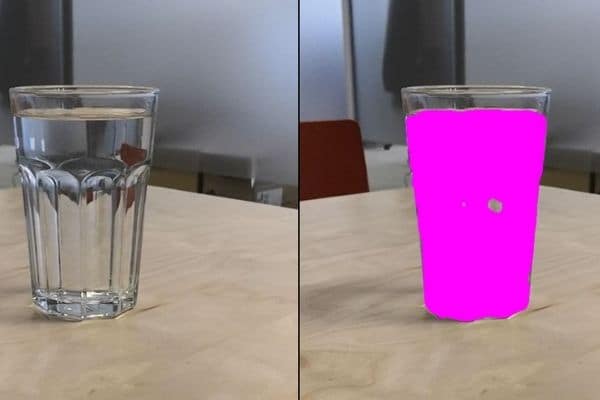
- Level detection of jars and bottles (for healthcare)
- Detection of anomalies in objects and people (for industry and healthcare)
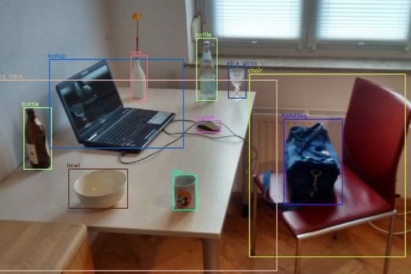
In the following we describe the procedure - from the greenfield to the trained model.
Benefits and challenges of spill detection
At a high level, the aim of the Use Case is to "Spillage detection to design a model that automatically detects industrial liquids on the floor as well as spills in healthcare facilities (e.g. nursing homes). In the future, robots will be equipped with this technology, which will enable them to locate puddles on the floor and thus avoid accidents by alerting maintenance staff. In addition, the robot itself should not be hindered by the liquid.
Spilled liquids on the floor are a potential danger for autonomous systems and people. Electronics can fail and people can slip and injure themselves. In addition, the liquid on the floor may have chemical, biological or otherwise hazardous components that should not be spread further. Robots currently used in industry and healthcare typically only detect an anomaly on the floor, stop and wait for a human to attend to the situation. Therefore, a model that can accurately detect the puddle, send an alarm and safely avoid the puddle can save a lot of time, reduce possible incidents and improve the operational flow smooth design. Nevertheless, the requirement to detect spills in different indoor environments presents the challenge of developing a model that has wide application.
The field of recognising objects on images through ML techniques is very well developed. What makes our use case so challenging? Why can't pre-trained models solve this problem inherently? Let us start with the general Difficulty begin. Spills vary in shape and colour and their texture is highly dependent on the environment. Additionally, the reflection of the puddle surface makes it difficult for out-of-the-box object recognition algorithms to learn correctly. An even more serious (and widespread in ML research) challenge is the fact that there is as yet no Labelled records for the detection of liquids indoors.
Data: A first starting point in ML projects
The investigation of state-of-the-art approaches for our use case points directly to data sets for autonomous driving, as self-driving cars also need to detect liquids on the ground. The Puddle 1000 record and the model developed by Australian researchers (https://github.com/Cow911/SingleImageWaterHazardDetectionWithRAU) have proven that image segmentation approaches are promising in terms of outdoor water puddle detection. The model used in this project was based on Reflection Attention Units with a TensorFlow setup in the background. We implemented a dynamic UNET of fast.ai on the Puddle-100 dataset as a first approach to this. Besides fast results, a valuable outcome of this approach was a better sense and understanding of the Nature of puddles: A major influence on puddles is the environment (e.g. through reflection), the perspective from which the images were taken and, above all, the exposure to light. Since all these properties are enormously different in outdoor and indoor scenarios, we decided that a new and self-produced data set, adapted to our indoor use case, was needed.
After we made this decision, many questions arose: What data do we need? How do we collect it? What metadata is valuable? As a starting point, we made a list of important Influencing factorswhich should be taken into account when recording video:
- Light (electric vs. natural, light vs. dark, shadow, position of light source)
- Background of the interior scene (colour and texture of the floor, natural reflections on dry floor, number and mobility of objects in the scene).
- Size/amount of spillage (no spillage, small stain vs. whole floor, one stain vs. many stains).
- Orientation of the camera (horizontal, view up vs. view down)
- Movement in the scene (standing vs. driving, change of direction)
- Type of puddle (water, coffee, coloured water to mimic dangerous liquids).
Therefore, we decided, Create videos that mimic robots in movements and use an evenly distributed medical and industrial background. The result was 51 videos, 30-60 seconds each, along with an Excel spreadsheet that compresses the metadata of each video.
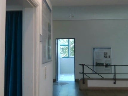
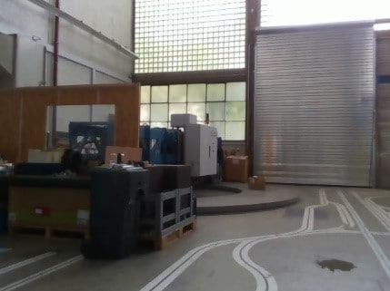
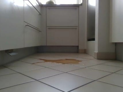
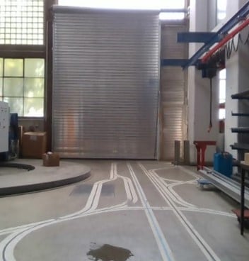
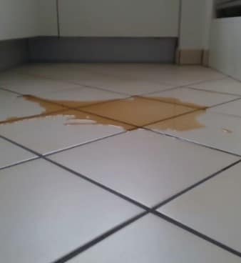
Middle: Water puddle in industrial hall, right: Coffee puddle on tiles
An important Lesson was that the distribution of the environmental variables must be clarified before recording begins in order to create a valuable data set for training a model for our specific use case.
The labelling of the data: Elaborate, but indispensable
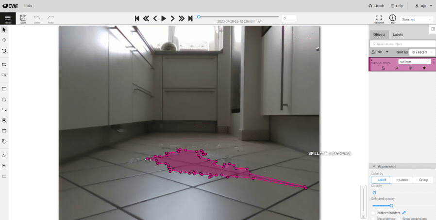
Now that we have our own dataset, the next big task for supervised learning is upon us: the labelling of the data! For segmentation tasks, this is the most important and elaborate part to make a dataset valuable. Since the requirement in our segmentation use case is to detect precise boundaries of the puddle, in each image we had to highly complex polygons draw. Due to the estimated high effort of labelling, we saw the need for a suitable platform where many people (not necessarily with deep domain knowledge, e.g. working students) can work together.
The result was the creation of a highly automated tool called CVAT (Computer Vision Annotation Tooldeveloped by Intel and OpenCV) with connection to a cloud server and storage. One advantage of this solution is that it can be deployed on the web and thus have an easy-to-use interface (can be run in a browser) for all users. Additionally, it allows for easy automation of tasks through the use of a Rest API. Learn more about this implementation in one of our future blog posts on labelling best practices!
How to find the right model
The first step before we start ML coding is to set up a Development environmentwhich supports collaborative working in rapid iterations enables and provides the basis for a scalable and reproducible solution. For the sake of simplicity, we have chosen to develop in Jupyter notebooks, which run on a On-Premise GPU Cluster hosted with four GPU nodes, each with ~12 GB of memory. The on-premise solution had two big advantages for us: lower costs in terms of cloud prices and time saved in onboarding new staff to the project. To ensure smooth teamwork, we introduced coding guidelines. This specifies that each ready-to-use function is stored in a Python module with Git tracking and a shared environment file is kept up to date to fix differing package versions.
Moving on to model development, we will focus on two main aspects: the Model selection and the Model tuning (although there are many more steps that need to be considered but are beyond the scope of this blog post).
Since the Fast.ai approach gave us fast and good results on the Puddle 100 dataset, we decided to start this use case on our own dataset as well and implement some further developments on it. We would like to present some important challenges and our results here:
- Thinking about a meaningful Test train distribution is important to be able to trust the results of the model training. We decided to distribute the backgrounds evenly between the test and train splits and also added a function (like the Blocking factor from the MLR package) is applied, which evenly distributes the images extracted from a video.
- For loss functions for segmentation tasks, it is recommended to use Focal Loss and Dice Loss (as informative reading: How to segment buildings on drone imagery ... ). It was very interesting that the use of the two best known loss functions - viz. Cross Entropy Loss and Binary Entropy Loss - gave us a scattered result (i.e. the puddle was detected but not in a coherent form).
- The right choice of Metrics is crucial when it comes to evaluation. We have defined various metric functions, such as dice_iou, accuracy, recall, negative_predicted_value, specificity and f1_score. All metrics are implemented on a pixel basis and on an image basis, e.g. a proportion of detected puddle pixels that were actually puddles vs. a proportion of predicted puddle images that were actually puddle images. For us, it made the most sense to take a closer look at the dice_iou metric.
- In addition to the numerical measurement, we found it helpful to use a less automated, but adapted validation function to have. Here we found that a comparison of ground truth and predicted masks grouped by metadata (e.g. background, industrial or not, buried or not) can be particularly useful to classify the performance of our training.
One of our biggest learnings from working with the fast.ai package was that it is an easy to use out-of-the-box approach, but when it comes to customisation and modification, it can get complicated quite quickly.
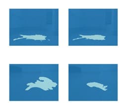
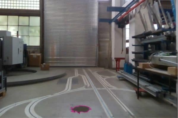
Function for the group background 'Hall' was output (left field: dressed truth, right field: prediction
When we were ready to train the model, important decisions had to be made about the Model architecture be met. We played around with different settings, but quickly decided on a U-Net architecture that builds well on the pre-trained encoder resnet18. U-Nets have become popular in recent years for image segmentation tasks. The idea comes from the paper "U-Net: Convolutional Networks for Biomedical Image Segmentation" by Olaf Ronneberger, Philipp Fischer and Thomas Brox from 2015. Briefly summarised, the idea of this architecture is to perform a downsampling routine on the input image, followed by a subsequent upsampling to restore the original input size. This enables the precise localisation of objects on the image. In addition, the architecture consists of a contracting path to capture context.
Model tuning
Our next step was the Tuning the hyperparameters. This task has two parts: testing the data extension and the model parameters. The biggest challenge here was to find an automated way to set the learning rate parameter correctly. In some samples of learning curves, we discovered many different shapes and a large impact of the choice of learning rate on the prediction accuracy. Therefore, we implemented three ways to find an "optimal" learning rate and included it as a parameter in the tuning:
- Minimal gradient: Select the learning rate that has the minimum gradient. This value can be taken directly from the function lr_find be taken over by fast.ai.
- Minimum Loss Shifted: The learning rate is determined like this: Find the minimum value and move it one tenth to the left. This approach is based on a kind of rule of thumb that goes back to Jeremy Howard (co-founder of fast.ai). This value can be determined (with a little extra effort) from the function lr_find be extracted from fast.ai.
- Appropriate Learning Rate: Since the previously mentioned direct ways to determine the learning rate do not work properly in some cases, we introduce a third approach based on a discussion in a fast.ai forum based. The idea is to construct a grid that is shifted from the right edge of the learning curve diagram to the left until a termination condition is met. This aims to obtain a learning rate that has a minimum loss gradient before the loss increases sharply. Note that with this approach, unique thresholds must be defined beforehand for each loss function used.
Once everything was set up, we performed a typical grid search in the parameter space shown in the following figure. For runtime reasons, we did this tuning on images that were resized to 25 %.

At each step, we saved the learning rate plot, the loss plot for test and validation data, the metric plots (most importantly for us, the dice_iou measure) and the validation images that we defined in the inspect results function described above. After running the hyperparameter training over a weekend, we can conclude with the following results:
- No clear "best values" for parameter tuning are recognisable.
- The value for "dice_iou" could be increased by approx. 5 % compared to the standard parameters.
- The "f1_score" could be raised by 2% to the standard parameter setting at the same time.
- It is difficult to compare results from different loss runs just by looking at the validation measures. Therefore, on some of the saved plots/measures, we performed a sample selection for the parameters with the highest accuracies. In doing so, we chose the following hyperparameter set (all other parameters are set to their default value):
Max_rotate=0,
max_zoom=1.4,
kind_of_lr='min_grade',
loss='dice_loss',
cycle_length=48
In summary, this time-consuming hyperparameter tuning did not give us the desired boost in model performance, but it did help us to better understand the model and provide the basis for automated training in a pipeline. As a final experiment for our Training process we have developed a procedure with iterative training with simultaneous Resizing the images implemented. The idea comes from Jeremy Howard (co-founder of fast.ai) from the fast.ai course, which can be taken online for free (https://course.fast.ai/). The idea behind this approach is that the model learns the overall behaviour of the segmentation shapes in the first runs (model training on a small image size). This allows the model to focus increasingly on the exact boundaries of the objects to be recognised in each loop. In our experiment, we started with downsized images of 25 %, scaled to 50 %, and then scaled to 75 % to finish training with the original image sizes. In each iteration, we manually adjusted the learning rate twice (each time after seeing the learning rate curve). To be able to transfer this training process into a final pipeline, we also implemented an automatic learning rate finder where the user can choose from the three automatic learning rate finding options described above (Minimal Gradient, Minimal Loss Shifted and Appropriate Learning Rate). The result of the dice_iou measure is the following:
| Image size | 0.25 | 0.5 | 0.75 | 1.0 |
|---|---|---|---|---|
| Evaluated on reduced images | 53,9% | 67,9% | 78,8% | 76,8% |
| Evaluated on full-size images | 22,6% | 55,6% | 73,2% | 76,8% |
This increase in accuracy can also be seen in the validation images. Therefore, this method seems to be very useful in our setup.
Summary and outlook
For us as data scientists, there is always a question in the background: How can we measure whether a model is good? What does the Accuracy value really? Are we looking at the right things? Of course, an accuracy of 77 % on our validation set tells us that the model is learning something. But is that enough? At this point it is good to go back to our initial motivation and the Real application to return to the task for which our model will be used: the recognition of puddles on the ground using assistive robots in care and industrial contexts. The puddle must be recognised and the boundaries of the overall shape should be clear, but it is not necessary for the shape to be 100 % correctly recognised, as would be the case in a task such as a robot grasping an object. As an intermediate implementation, the robot could stop and send an alarm when it detects a puddle. Clearly, in our use case, a false positive (detecting a puddle when there is none) is less fatal than not detecting the puddle and still spreading the unwanted liquid.
In evaluating whether our model was working "well", one answer for us was to selectively pick out some images in a clever way. Firstly, we looked at the images grouped by our collected metadata and secondly, we found it helpful to merge the images back with the original videos to see the predictive behaviour when the video was played. We would like to leave it to the reader to judge such an output:
In summary, we can say that the first results for our use case look very promising. Puddles are detected in most cases and a comprehensible trend can be seen in the videos. Of course, as always, there is room for improvement that can be addressed in the future. Our next steps are to test the model on additional data (which is currently being recorded) and test how well our model can be generalised, and then implement the model in the robotic system and test it in the real world.






0 Kommentare